
Analyzing Microbial Communities with R: A Comprehensive Workflow
Introduction
Microbial community analysis is a crucial aspect of environmental and clinical studies. In this blog post, we’ll walk through a complete workflow using R to process sequencing data, perform denoising, construct phylogenetic trees, and visualize the results. We will use several powerful packages, including ggplot2, phyloseq, dada2, phangorn, and DECIPHER, to achieve these tasks.
Workflow Overview
- Preprocessing and Quality Control
- Denoising and Merging Reads
- Taxonomy Assignment
- Phylogenetic Tree Construction
- Visualization
1. Preprocessing and Quality Control
The first step is to preprocess and filter your sequencing data. We use the dada2 package for this purpose, which provides tools for filtering, trimming, and quality control.
# Load required libraries
library(dada2)

# Set paths
seq_path <- "/Users/j/Downloads/project/fastq"
filt_path <- "/Users/j/Downloads/project/filtered_fastq"

# Preprocessing: Filter and trim sequences
fns <- sort(list.files(seq_path, full.names = TRUE))
fnFs <- fns[grepl("pass_1", fns)]
fnRs <- fns[grepl("pass_2", fns)]

if (!file_test("-d", filt_path)) dir.create(filt_path)
filtsFs <- file.path(filt_path, basename(fnFs))
filtsRs <- file.path(filt_path, basename(fnRs))
for (i in seq_along(fnFs)) {
  fastqPairedFilter(c(fnFs[i], fnRs[i]),
                    c(filtsFs[i], filtsRs[i]),
                    trimLeft = 10, truncLen = c(245, 160),
                    maxN = 0, maxEE = 2, truncQ = 2,
                    compress = TRUE)
}
Here, fastqPairedFilter is used to trim and filter the sequences, which helps in removing low-quality reads and adapters.
2. Denoising and Merging Reads
Next, we denoise the sequences and merge paired-end reads. This step helps in reducing errors and assembling the reads into contiguous sequences.
# Denoising and merging paired-end reads
derepFs <- derepFastq(filtsFs)
derepRs <- derepFastq(filtsRs)
sam.names <- sapply(strsplit(basename(filtsFs), "_"), `[`, 1)
names(derepFs) <- sam.names
names(derepRs) <- sam.names

ddF <- dada(derepFs, err=NULL, selfConsist=TRUE)
ddR <- dada(derepRs, err=NULL, selfConsist=TRUE)

dadaFs <- dada(derepFs, err=ddF[[1]]$err_out, pool=TRUE)
dadaRs <- dada(derepRs, err=ddR[[1]]$err_out, pool=TRUE)
mergers <- mergePairs(dadaFs, derepFs, dadaRs, derepRs)
seqtab <- makeSequenceTable(mergers)
dada performs error correction, and mergePairs assembles the paired-end reads into a single sequence table.
3. Taxonomy Assignment
Once the sequences are assembled, the next step is to assign taxonomy to the sequences. This helps in identifying the microbial taxa present in the samples.
# Assign taxonomy using reference database
library(DECIPHER)

ref_fasta <- "/Users/j/Downloads/rdp_train_set_14.fa.gz"
taxtab <- assignTaxonomy(seqtab, refFasta = ref_fasta)
colnames(taxtab) <- c("Kingdom", "Phylum", "Class", "Order", "Family", "Genus")
assignTaxonomy uses a reference database to classify the sequences.
4. Phylogenetic Tree Construction
Constructing a phylogenetic tree helps in understanding the evolutionary relationships between the microbial taxa.
# Construct phylogenetic tree
library(phangorn)

seqs <- getSequences(seqtab)
names(seqs) <- seqs # This propagates to the tip labels of the tree
alignment <- AlignSeqs(DNAStringSet(seqs), anchor=NA)
phang.align <- phyDat(as(alignment, "matrix"), type="DNA")
dm <- dist.ml(phang.align)
treeNJ <- NJ(dm)
fit <- pml(treeNJ, data=phang.align)
fitGTR <- update(fit, k=4, inv=0.2)
Here, AlignSeqs aligns the sequences, and NJ constructs the neighbor-joining tree.
5. Visualization
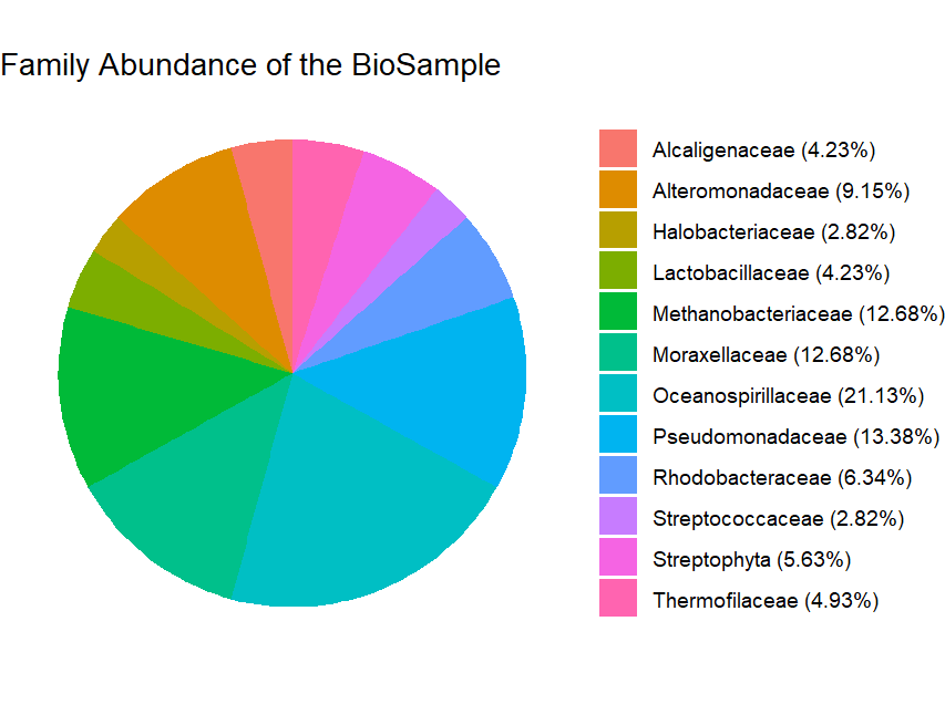
dat Finally, visualize the abundance of different taxa using a pie chart to gain insights into the microbial community composition.
# Load required libraries
library(phyloseq)
library(ggplot2)

# Load metadata and create phyloseq object
mimarks_path <- "/Users/j/Downloads/project/metadata.csv"
RDS_path <- "/Users/j/Downloads/project/ps.Rds"

samdf <- read.csv(mimarks_path, header=TRUE)
rownames(samdf) <- samdf$Run
ps <- phyloseq(tax_table(taxtab), sample_data(samdf),
               otu_table(seqtab, taxa_are_rows = FALSE), phy_tree(fitGTR$tree))

# Save the phyloseq object to a file
saveRDS(ps, file = RDS_path)

# Load the phyloseq object (if needed)
ps <- readRDS(RDS_path)

# Transform to relative abundance
ps_abund <- transform_sample_counts(ps, function(x) x)

# Melt the phyloseq object to a long format DataFrame
ps_melt <- psmelt(ps_abund)

# Filter LifeStage (e.g., "gut")
selected_data <- subset(ps_melt, ScientificName == "biofilm metagenome")

# Summarize abundance
by <- "Family"
order_abundance <- aggregate(reformulate(by, "Abundance"), data = selected_data, sum)

# Sort by abundance and filter out low abundance orders
order_abundance <- order_abundance[order(order_abundance$Abundance, decreasing = TRUE), ]
order_abundance$fract <- round(order_abundance$Abundance / sum(order_abundance$Abundance) * 100, 2)
order_abundance <- order_abundance[order_abundance$fract >= 2, ]

# Add labels for the pie chart
order_abundance$Label <- paste0(order_abundance[[by]], " (", round(order_abundance$Abundance / sum(order_abundance$Abundance) * 100, 2), "%)")

# Create and display the pie chart
ggplot(order_abundance, aes(x = "", y = Abundance, fill = Label)) +
  geom_bar(width = 1, stat = "identity") +
  coord_polar("y", start = 0) +
  theme_void() +
  labs(title = paste(by,"Abundance of the BioSample")) +
  theme(legend.title = element_blank())
The ggplot2 package is used to create a pie chart of the relative abundance of different families, providing a visual representation of the microbial community composition.
Conclusion
This workflow integrates several R packages to process and analyze sequencing data, construct phylogenetic trees, and visualize microbial community data. By following these steps, you can effectively manage and interpret complex biological datasets, making informed decisions in your research.
Appendix: Downloading SRR Files and Reference Data
Downloading SRR Files Using Python
To process sequencing data, you often need to download SRA (Sequence Read Archive) files. Below is a bash script to fetch SRA files using their SRR (Sequence Read Run) IDs. This script assumes you have the necessary tools installed, such as prefetch and fastq-dump from the SRA Toolkit.
# Bash. Define SRR IDs
ids=("SRR30211628" "SRR30211640" "SRR30211639" "SRR30211638" "SRR30211637"
    "SRR30211636" "SRR30211642" "SRR30211641" "SRR30211632" "SRR30211635"
    "SRR30211631" "SRR30211630" "SRR30211629" "SRR30211634" "SRR30211633"
)

# Define the directory to store FASTQ files
FASTQ_DIR="/content/fastqs"

# Create the output directory if it doesn't exist
mkdir -p "${FASTQ_DIR}"

# Loop through each SRR ID
for id in "${ids[@]}"; do
    echo "Processing ${id}..."

    # Define SRA file path
    sra_file="/content/${id}/${id}.sra"

    # Download the SRA file if it doesn't exist
    if [ ! -f "${sra_file}" ]; then
        echo "Prefetching ${id}..."
        prefetch ${id} &>/dev/null
    else
        echo "SRA file already exists for ${id}"
    fi

    # Run fastq-dump
    echo "Running fastq-dump for ${id}..."
    fastq-dump --outdir "${FASTQ_DIR}" --gzip --skip-technical --readids --read-filter pass --dumpbase --split-3 --clip "${sra_file}" &>/dev/null
done

echo "All downloads complete."
Using the Reference Database
For taxonomy assignment, a reference database is required. You can use the RDP (Ribosomal Database Project) training set for this purpose. The training set can be downloaded from the following GitHub repository:
Download the file and save it to your local directory. Make sure the path to this file is correctly specified in your R script:
ref_fasta <- "/Users/j/Downloads/project/rdp_train_set_14.fa.gz"
By using this reference database, you can accurately assign taxonomy to your sequence data, ensuring reliable results in your microbial community analysis.
To download and save run information from NCBI’s SRA database as metadata.csv, follow these steps:
Download the Metadata from NCBI
You can download the run information manually from the NCBI website or automate the process using a script. Here’s how you can do it using Python:
Manual Download
- Go to the NCBI SRA page.
- On the page, look for the “Send to” button or similar options to export data.
- Choose to export in CSV format and download the file.
Conclusion
This appendix provides essential steps for obtaining SRR files and the necessary reference data. Proper downloading and management of these files are crucial for accurate and efficient data analysis in microbial studies.
