Building an XGBoost Classifier with Margin Scores in Python

Background

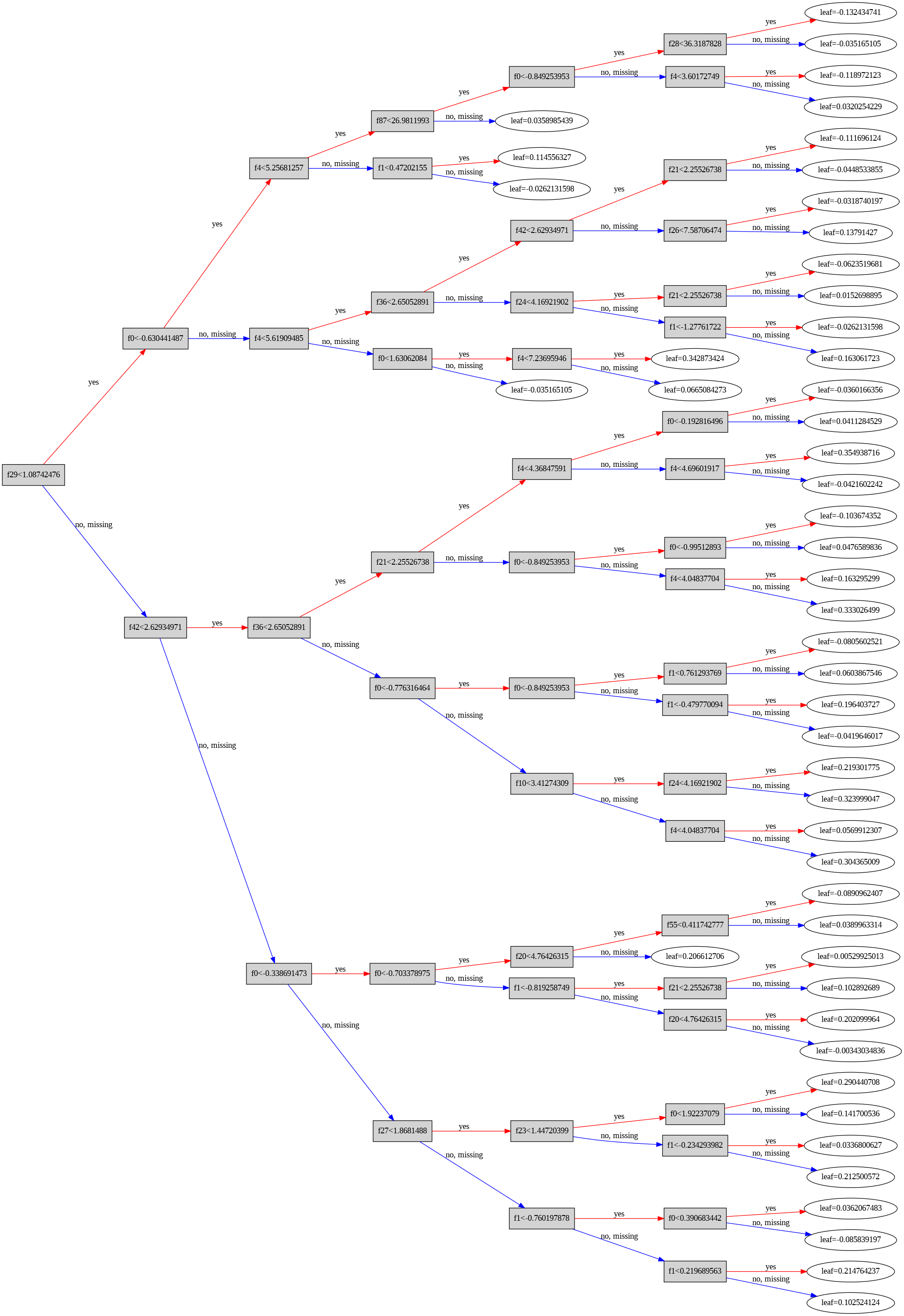
XGBoost, which stands for Extreme Gradient Boosting, is an advanced implementation of gradient boosting, a powerful machine learning technique. XGBoost has gained significant popularity in the data science community due to its efficiency, speed, and high performance. It is designed to be highly scalable and supports parallel and distributed computing, making it suitable for large datasets and complex problems. XGBoost operates by creating an ensemble of weak decision trees, which are sequentially added to correct the errors made by the previous trees. This iterative process enhances the model’s accuracy and generalization capabilities. Key features of XGBoost include regularization to prevent overfitting, handling of missing values, and the ability to optimize a wide range of objective functions. These attributes have made XGBoost a top choice for winning machine learning competitions and for solving real-world predictive analytics problems.

In this blog, we will walk through a complete machine learning pipeline using XGBoost to predict income levels based on the UCI Adult dataset. We’ll cover data loading, preprocessing, model training, evaluation, and visualization. The unique aspect of this pipeline is the use of margin scores to improve model evaluation.

Step 1: Import Libraries

First, we need to import the necessary libraries for data manipulation, preprocessing, model training, and evaluation.

import numpy as np
import xgboost as xgb
from sklearn.model_selection import train_test_split
from sklearn.preprocessing import StandardScaler
from sklearn.datasets import fetch_openml
import pandas as pd
from sklearn.metrics import accuracy_score, precision_score, recall_score, f1_score

Step 2: Define XGBoost Parameters

We’ll define a function to return the XGBoost parameters.

def xgboost_plst():
    param = {
        'max_depth': 6,                # Depth of tree
        'eta': 0.1,                    # Learning rate
        'objective': 'binary:logistic',
        'nthread': 7,                  # Number of threads used
        'eval_metric': 'logloss',
        'subsample': 0.8,              # Subsample ratio of the training instance
        'colsample_bytree': 0.8,       # Subsample ratio of columns when constructing each tree
        'gamma': 0.1,                  # Minimum loss reduction required to make a further partition
        'lambda': 1,                   # L2 regularization term on weights
        'alpha': 0                     # L1 regularization term on weights
    }
    return param

Step 3: Load and Preprocess the Dataset

Next, we load the dataset from the UCI repository and preprocess it. This includes one-hot encoding categorical features and standardizing numerical features.

# Load the dataset from UCI repository
adult_data = fetch_openml(name='adult', version=2, as_frame=True)
X = adult_data.data
y = adult_data.target

# Convert target to binary (<=50K -> 0, >50K -> 1)
y = (y == '>50K').astype(int).to_numpy()

# One-hot encode categorical features
X = pd.get_dummies(X, drop_first=True)

# Standardize the features
scaler = StandardScaler(with_mean=True)
X = scaler.fit_transform(X)

# Split the data into training and test sets
X_train, X_test, y_train, y_test = train_test_split(X, y, test_size=0.2, random_state=42)

Step 4: Define a Function to Calculate Statistics for Margin Scores

We’ll define a function to calculate statistics (mean and standard deviation) for margin scores, which helps in evaluating model performance.

def calc_stats(margin_scores):
    mean_scores = np.mean(margin_scores, axis=1)
    std_scores = np.std(margin_scores, axis=1)

    min_scr = mean_scores - 3 * std_scores
    max_scr = mean_scores + 3 * std_scores

    min_scr = np.round(min_scr, 2)
    max_scr = np.round(max_scr, 2)

    return min_scr, max_scr

Step 5: Train the Model and Calculate Margin Scores

We create a function that trains the XGBoost model using bootstrapping, computes margin scores, and evaluates the model.

def process(X_train, X_test, y_train, y_test, n_bootstrap=100):
    margin_scores = []

    for i in range(n_bootstrap):
        indices = np.random.choice(X_train.shape[0], X_train.shape[0], replace=True)
        X_sample = X_train[indices,:]
        y_sample = y_train[indices]

        dtrain = xgb.DMatrix(X_sample, label=y_sample)
        dtest = xgb.DMatrix(X_test, label=y_test)

        evallist = [(dtrain, 'train'), (dtest, 'eval')]

        bst = xgb.train(xgboost_plst(), dtrain, num_boost_round=100, evals=evallist, verbose_eval=False)

        preds = bst.predict(dtest, output_margin=True)
        margin_scores.append(preds)

    margin_scores = np.array(margin_scores).T

    min_scr, max_scr = calc_stats(margin_scores)

    # Convert margin scores to predictions
    pred = np.where(max_scr < 0, 0, np.where(min_scr >= 0, 1, 2))

    # Evaluate performance
    accuracy = accuracy_score(y_test, pred)
    print("Accuracy:", accuracy)

    return min_scr, max_scr, pred

Step 6: Run the Process Function

We run the process function on our dataset to get the minimum and maximum margin scores and predictions.

# Run the process function on the dataset
min_scr, max_scr, pred = process(X_train, X_test, y_train, y_test)

Step 7: Evaluate Model Performance

Finally, we define a function to evaluate the model performance using a confusion matrix and ROC curve, then visualize the results.

from sklearn.metrics import confusion_matrix, roc_curve, auc
from sklearn.metrics import confusion_matrix, ConfusionMatrixDisplay
import matplotlib.pyplot as plt

# Function to evaluate model performance
def evaluate_performance(y_true, y_pred):
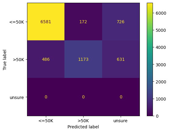
    # Confusion matrix
    cm = confusion_matrix(y_true, y_pred)
    disp = ConfusionMatrixDisplay(confusion_matrix=cm, display_labels=["<=50K", ">50K", "unsure"])
    disp.plot()

    # ROC curve
    fpr, tpr, thresholds = roc_curve(y_true, y_pred)
    roc_auc = auc(fpr, tpr)

    plt.figure()
    plt.plot(fpr, tpr, color='darkorange', lw=2, label='ROC curve (area = %0.2f)' % roc_auc)
    plt.plot([0, 1], [0, 1], color='navy', lw=2, linestyle='--')
    plt.xlim([0.0, 1.0])
    plt.ylim([0.0, 1.05])
    plt.xlabel('False Positive Rate')
    plt.ylabel('True Positive Rate')
    plt.title('Receiver Operating Characteristic (ROC)')
    plt.legend(loc="lower right")
    plt.show()

# Evaluate performance
evaluate_performance(y_test, pred)

Conclusion

This blog post demonstrated how to build and evaluate an XGBoost classifier on the UCI Adult dataset. By using margin scores, we introduced a method to better understand and interpret model predictions, which can be particularly useful in binary classification problems. The complete pipeline included data loading, preprocessing, model training, evaluation, and visualization, providing a comprehensive guide for working with similar datasets and models.